12 - S Curve Trajectory
System in Analysis
The complete example code is available here.
The mechanical powertrain to be studied is reported in the image below:
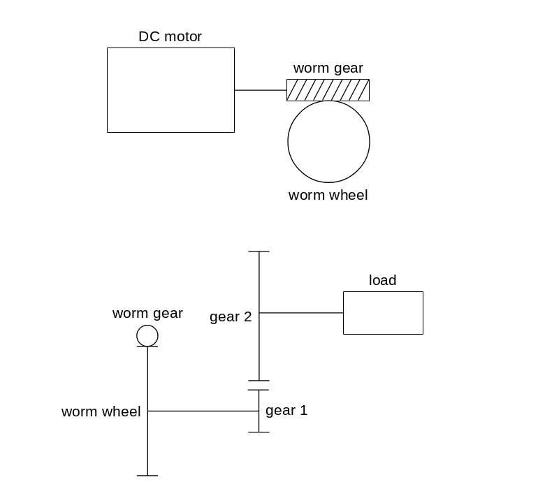
The worm gear is connected to the DC motor output shaft and rotates with
it. The worm gear mates with the worm wheel, which is connected to gear 1
through a rigid shaft, so the worm wheel and the gear 1 rotate together.
Finally, the gear 2 mates with gear 1 and carries the external load.
The analysis is focused on final gear 2 position and velocity control with
respect to an S-curve trajectory from a starting to a stopping positions.
Model Set Up
As a first step, we instantiate the components of the mechanical powertrain:
from gearpy.mechanical_objects import DCMotor, WormGear, WormWheel, SpurGear
from gearpy.units import (
    AngularSpeed,
    InertiaMoment,
    Torque,
    Current,
    Angle,
)

motor = DCMotor(
    name='motor',
    no_load_speed=AngularSpeed(value=3000, unit='rpm'),
    maximum_torque=Torque(value=2000, unit='gfcm'),
    inertia_moment=InertiaMoment(value=50, unit='gcm^2'),
    no_load_electric_current=Current(value=0, unit='mA'),
    maximum_electric_current=Current(value=5, unit='A')
)
worm_gear = WormGear(
    name='worm gear',
    n_starts=1,
    inertia_moment=InertiaMoment(value=1, unit='gcm^2'),
    pressure_angle=Angle(value=20, unit='deg'),
    helix_angle=Angle(value=10, unit='deg')
)
worm_wheel = WormWheel(
    name='worm wheel',
    n_teeth=50,
    inertia_moment=InertiaMoment(value=40, unit='gcm^2'),
    pressure_angle=Angle(value=20, unit='deg'),
    helix_angle=Angle(value=10, unit='deg')
)
gear_1 = SpurGear(
    name='gear 1',
    n_teeth=10,
    inertia_moment=InertiaMoment(value=2, unit='gcm^2')
)
gear_2 = SpurGear(
    name='gear 2',
    n_teeth=40,
    inertia_moment=InertiaMoment(value=100, unit='gcm^2')
)
Then it is necessary to specify the connection types between the components. We choose to study a non-ideal powertrain so, in order to take into account power loss in mating due to friction, we specify a gear mating efficiency below \(100\%\) and a friction coefficient in the worm gear mating:
from gearpy.utils import add_fixed_joint, add_gear_mating, add_worm_gear_mating

add_fixed_joint(master=motor, slave=worm_gear)
add_worm_gear_mating(
    master=worm_gear,
    slave=worm_wheel,
    friction_coefficient=0.2
)
add_fixed_joint(master=worm_wheel, slave=gear_1)
add_gear_mating(master=gear_1, slave=gear_2, efficiency=0.9)
We have to define the external load applied to gear 2. The load torque is periodic with respect to the final gear angular position:
def ext_torque(time, angular_position, angular_speed):
    return Torque(
        value=3*(1-angular_position.cos(frequency=2)),
        unit='Nm'
    )

gear_2.external_torque = ext_torque
Then we have to define the S-curve trajectory characteristics and the control
logic to apply to the motor, in order to make the gear 2 follow a specific
trajectory.
The gear 2 starts from \(0\ rad\) and stops to \(1.5\ rad\) for few seconds, then
goes back to \(1\ rad\) as final position; these values are going to be multiplied
by the total reduction ratio to get the respective motor positions.
To properly reproduce the three motion phases, we can split each of them in
three analysis:
a forward motion of the gear 2 from \(0\ rad\) to \(1.5\ rad\)
a pause at \(1.5\ rad\)
a backward motion of the gear 2 from \(1.5\ rad\) to \(1\ rad\)
We can define these reference positions:
from grerpy.units import AngularPosition

start_position = AngularPosition(value=0, unit='rad')
intermediate_position = AngularPosition(value=1.5, unit='rad')
final_position = AngularPosition(value=1, unit='rad')
With respective to the motor, the forward and backward motions are determined by the S-curve, which has 3 parts:
an acceleration part at \(200\ rad/s^2\)
a steady velocity part at \(150\ rad/s\)
a deceleration part at \(120\ rad/s^2\)
We can proceed to define the trajectory of the motor in the first phase:
from gearpy.units import AngularAcceleration
from gearpy.motor_control.utils import SCurveTrajectory

total_reduction_ratio = gear_2.n_teeth/gear_1.n_teeth*worm_wheel.n_teeth

start_speed = AngularSpeed(value=0, unit='rad/s')


trajectory = SCurveTrajectory(
    start_position=total_reduction_ratio*start_position,
    stop_position=total_reduction_ratio*intermediate_position,
    maximum_velocity=AngularSpeed(value=150, unit='rad/s'),
    maximum_acceleration=AngularAcceleration(value=200, unit='rad/s^2'),
    maximum_deceleration=AngularAcceleration(value=120, unit='rad/s^2'),
    start_velocity=total_reduction_ratio*start_speed,
)
See SCurveTrajectory
for more details on the S-curve trajectory.
Then we can define the control tool the make the motor follow the trajectory: a
position and velocity control made by two nested PID controllers. The position
PID generates a velocity reference used by the velocity PID to compute a PWM
reference:
from gearpy.motor_control.utils import PIDController

position_PID = PIDController(Kp=40, Ki=50, Kd=0)
velocity_PID = PIDController(
    Kp=0.002,
    Ki=0.2,
    Kd=0,
    clamping=True,
    reference_min=-1,
    reference_max=1
)
See PIDController
for more details on PID controllers.
Finally, we can combine all components in a powertrain object and define the
control logic:
from gearpy.powertrain import Powertrain
from gearpy.sensors import AbsoluteRotaryEncoder, Tachometer
from gearpy.motor_control.rules import PositionAndVelocityControl
from gearpy.motor_control import PWMControl

powertrain = Powertrain(motor=motor)

encoder = AbsoluteRotaryEncoder(target=motor)
tachometer = Tachometer(target=motor)

position_control = PositionAndVelocityControl(
    encoder=encoder,
    tachometer=tachometer,
    powertrain=powertrain,
    position_PID=position_PID,
    velocity_PID=velocity_PID,
    trajectory=trajectory
)

motor_control = PWMControl(powertrain=powertrain)
motor_control.add_rule(rule=position_control)
See PositionAndVelocityControl
for more details on this specific PWM control rule.
First Phase Simulation Set Up
Before performing the simulation, it is necessary to set the initial condition of the system in terms of angular position and speed of the last gear in the mechanical powertrain:
gear_2.angular_position = start_position
gear_2.angular_speed = start_speed
Additionally, we can define a stop condition, to terminate the computation as soon as the gear 2 reaches the desired stop position:
from gearpy.utils import StopCondition

intermediate_stop_condition = StopCondition(
    sensor=encoder,
    threshold=total_reduction_ratio*intermediate_position,
    operator=StopCondition.greater_than_or_equal_to
)
Finally, we have to set up the simulation parameters: the time discretization
for the time integration and the simulation time; notice the simulation_time
set to \(1\ min\) to let the solver run up until the stop condition to occur.
Now we are ready to run the simulation:
from gearpy.units import TimeInterval
from gearpy.solver import Solver


time_step = TimeInterval(value=0.0001, unit="sec")

solver = Solver(powertrain=powertrain)
solver.run(
    time_discretization=time_step,
    simulation_time=TimeInterval(value=1, unit='min'),
    motor_control=motor_control,
    stop_condition=intermediate_stop_condition
)
First Phase Results Analysis
We can get a plot of the motor and gear 2 time variables:
powertrain.plot(
    figsize=(8, 10),
    elements=['motor', 'gear 2'],
    variables=[
        'angular position',
        'angular speed',
        'angular acceleration',
        'driving torque',
        'load torque',
        'torque',
        'electric current',
        'pwm'
    ]
)
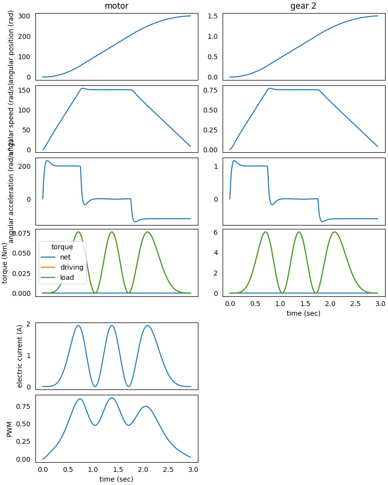
We can see that the gear 2 does not properly follow the trajectory in terms of quickness: the accelerations reach the set values too slowly. So, we have to re-define the position PID controller to get better performances:
position_PID = PIDController(Kp=4000, Ki=50, Kd=0)
velocity_PID.reset()

position_control = PositionAndVelocityControl(
    encoder=encoder,
    tachometer=tachometer,
    powertrain=powertrain,
    position_PID=position_PID,
    velocity_PID=velocity_PID,
    trajectory=trajectory
)

motor_control = PWMControl(powertrain=powertrain)
motor_control.add_rule(rule=position_control)

powertrain.reset()

solver.run(
    time_discretization=time_step,
    simulation_time=TimeInterval(value=1, unit='min'),
    motor_control=motor_control,
    stop_condition=intermediate_stop_condition
)

powertrain.plot(
    figsize=(8, 10),
    elements=['motor', 'gear 2'],
    variables=[
        'angular position',
        'angular speed',
        'angular acceleration',
        'driving torque',
        'load torque',
        'torque',
        'electric current',
        'pwm'
    ]
)
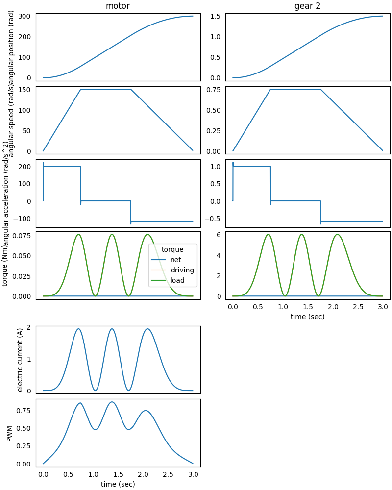
We can appreciate the better performances of this motor control in terms of trajectory.
Following Phases Simulation Set Up
Now we can proceed with the second phase: the pause at \(1.5\ rad\) with a constant PWM to keep the system still in position:
from gearpy.sensors import Timer
from gearpy.motor_control.rules import ConstantPWM

timer = Timer(
    start_time=powertrain.time[-1],
    duration=TimeInterval(value=1.1, unit='sec'),
)

keep_position = ConstantPWM(
    timer=timer,
    powertrain=powertrain,
    target_pwm_value=0
)

motor_control = PWMControl(powertrain=powertrain)
motor_control.add_rule(rule=keep_position)


solver = Solver(powertrain=powertrain)
solver.run(
    time_discretization=time_step,
    simulation_time=TimeInterval(value=1, unit='sec'),
    motor_control=motor_control,
)

powertrain.plot(
    figsize=(8, 10),
    elements=['motor', 'gear 2'],
    variables=[
        'angular position',
        'angular speed',
        'angular acceleration',
        'driving torque',
        'load torque',
        'torque',
        'electric current',
        'pwm'
    ]
)
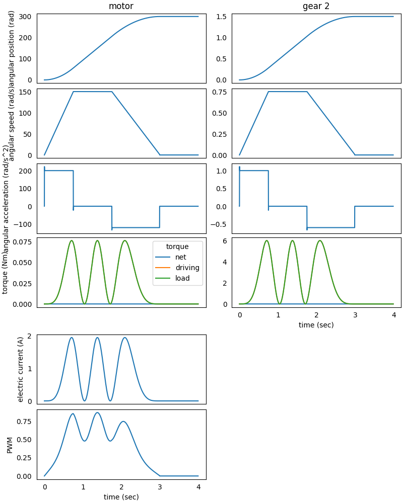
Now we can model the third and final phase: the backward motion from \(1.5\ rad\)
to \(1\ rad\) with the respective S-curve trajectory.
Firstly, we have to invert the external torque sign to keep the external load
coherent:
def ext_torque(time, angular_position, angular_speed):
    return Torque(
        value=-3*(1-angular_position.cos(frequency=2)),
        unit='Nm'
    )

gear_2.external_torque = ext_torque
Then we can proceed with the backward motion:
trajectory = SCurveTrajectory(
    start_position=motor.angular_position,
    stop_position=total_reduction_ratio*final_position,
    maximum_velocity=AngularSpeed(value=150, unit='rad/s'),
    maximum_acceleration=AngularAcceleration(value=200, unit='rad/s^2'),
    maximum_deceleration=AngularAcceleration(value=120, unit='rad/s^2'),
    start_velocity=motor.angular_speed,
    start_time=powertrain.time[-1]
)

position_PID.reset()
velocity_PID.reset()

position_control = PositionAndVelocityControl(
    encoder=encoder,
    tachometer=tachometer,
    powertrain=powertrain,
    position_PID=position_PID,
    velocity_PID=velocity_PID,
    trajectory=trajectory
)

motor_control = PWMControl(powertrain=powertrain)
motor_control.add_rule(rule=position_control)

final_stop_condition = StopCondition(
    sensor=encoder,
    threshold=total_reduction_ratio*final_position,
    operator=StopCondition.less_than_or_equal_to
)

solver = Solver(powertrain=powertrain)
solver.run(
    time_discretization=time_step,
    simulation_time=TimeInterval(value=1, unit='min'),
    motor_control=motor_control,
    stop_condition=final_stop_condition
)

powertrain.plot(
    figsize=(8, 10),
    elements=['motor', 'gear 2'],
    variables=[
        'angular position',
        'angular speed',
        'angular acceleration',
        'driving torque',
        'load torque',
        'torque',
        'electric current',
        'pwm'
    ]
)
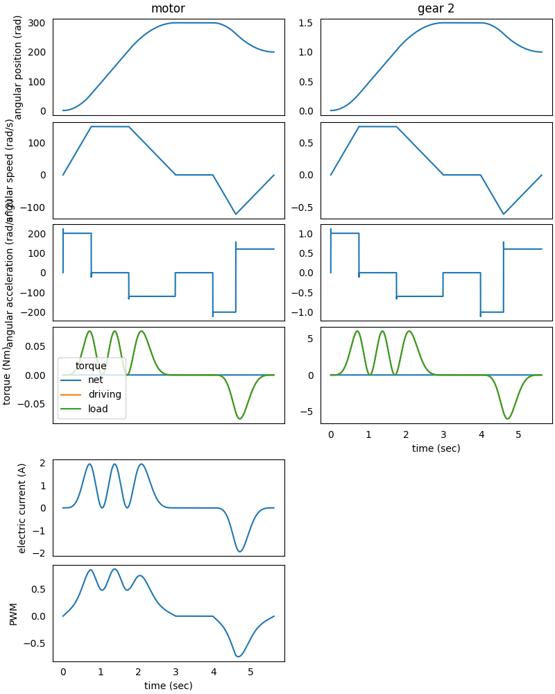
We can see that, in this case, there is no room for a uniform velocity step: the motor goes directly from the acceleration part to the deceleration part.