System in Analysis
The complete example code is available
here.
The mechanical powertrain to be studied is reported in the image below:
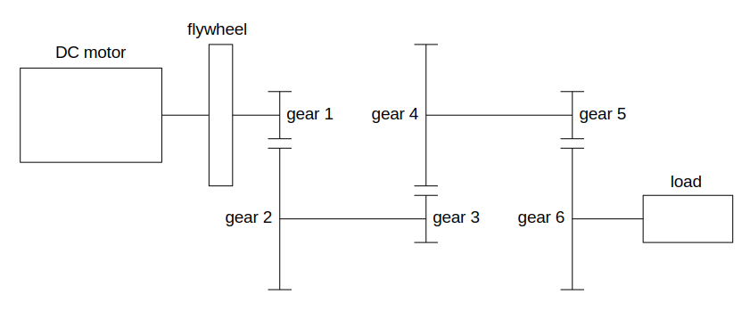
The flywheel and the gear 1 are connected to the DC motor output
shaft and rotate with it. The gear 2 mates with gear 1 and is
connected to gear 3 through a rigid shaft, so gear 2 and gear 3
rotate together. The gear 3 mates with gear 4, to which is connected
to gear 5 through another rigid shaft, so gear 4 and gear 5 rotate
together. Finally, gear 5 mates with gear 6, which is connected to
the external load.
The analysis is focused on powertrain elements kinematics and torques.
Model Set Up
As a first step, we instantiate the components of the mechanical powertrain:
from gearpy.mechanical_objects import DCMotor, Flywheel, SpurGear
from gearpy.units import AngularSpeed, InertiaMoment, Torque

motor = DCMotor(
    name='motor',
    no_load_speed=AngularSpeed(15000, 'rpm'),
    maximum_torque=Torque(10, 'mNm'),
    inertia_moment=InertiaMoment(3, 'gcm^2')
)
flywheel = Flywheel(
    name='flywheel',
    inertia_moment=InertiaMoment(20, 'kgcm^2')
)
gear_1 = SpurGear(
    name='gear 1',
    n_teeth=10,
    inertia_moment=InertiaMoment(1, 'gcm^2')
)
gear_2 = SpurGear(
    name='gear 2',
    n_teeth=80,
    inertia_moment=InertiaMoment(3100, 'gcm^2')
)
gear_3 = SpurGear(
    name='gear 3',
    n_teeth=10,
    inertia_moment=InertiaMoment(4, 'gcm^2')
)
gear_4 = SpurGear(
    name='gear 4',
    n_teeth=60,
    inertia_moment=InertiaMoment(5000, 'gcm^2')
)
gear_5 = SpurGear(
    name='gear 5',
    n_teeth=10,
    inertia_moment=InertiaMoment(12, 'gcm^2')
)
gear_6 = SpurGear(
    name='gear 6',
    n_teeth=50,
    inertia_moment=InertiaMoment(7600, 'gcm^2')
)
See DCMotor,
Flywheel and
SpurGear for
more details on instantiation parameters.
Then it is necessary to specify the connection types between the
components. We choose to study a non-ideal powertrain so, in order to
take into account power loss in mating due to friction, we specify a
\(90\%\) gear mating efficiency:
from gearpy.utils import add_fixed_joint, add_gear_mating

add_fixed_joint(master=motor, slave=flywheel)
add_fixed_joint(master=flywheel, slave=gear_1)
add_gear_mating(master=gear_1, slave=gear_2, efficiency=0.9)
add_fixed_joint(master=gear_2, slave=gear_3)
add_gear_mating(master=gear_3, slave=gear_4, efficiency=0.9)
add_fixed_joint(master=gear_4, slave=gear_5)
add_gear_mating(master=gear_5, slave=gear_6, efficiency=0.9)
See add_fixed_joint
and add_gear_mating
for more details.
We have to define the external load applied to gear 6. To keep the
example simple, we can consider a constant load torque:
def ext_torque(time, angular_position, angular_speed):
    return Torque(500, 'mNm')


gear_6.external_torque = ext_torque
Finally, it is necessary to combine all components in a powertrain object:
from gearpy.powertrain import Powertrain

powertrain = Powertrain(motor=motor)
See Powertrain for more
details on this class and its methods.
Simulation Set Up
Before performing the simulation, it is necessary to specify the initial condition of the system in terms of angular position and speed of the last gear in the mechanical powertrain. In this case we can consider the gear 6 still in the reference position:
from gearpy.units import AngularPosition

gear_6.angular_position = AngularPosition(0, 'rad')
gear_6.angular_speed = AngularSpeed(0, 'rad/s')
Finally, we have to set up the simulation parameters: the time discretization for the time integration and the simulation time. Now we are ready to run the simulation::
from gearpy.units import TimeInterval
from gearpy.solver import Solver

solver = Solver(powertrain=powertrain)
solver.run(
    time_discretization=TimeInterval(0.5, 'sec'),
    simulation_time=TimeInterval(20, 'sec')
)
See Solver for more details.
Results Analysis
We can get a snapshot of the system at a particular time of interest:
from gearpy.units import Time

powertrain.snapshot(target_time=Time(10, 'sec'))
Mechanical Powertrain Status at Time = 10 sec
          angular position (rad)  angular speed (rad/s)  angular acceleration (rad/s^2)  torque (Nm)  driving torque (Nm)  load torque (Nm)  pwm
motor                9714.908984            1119.894923                        1.085094     0.000013             0.002871          0.002858  1.0
flywheel             9714.908984            1119.894923                        1.085094     0.000013             0.002871          0.002858
gear 1               9714.908984            1119.894923                        1.085094     0.000013             0.002871          0.002858
gear 2               1214.363623             139.986865                        0.135637     0.000092             0.020668          0.020576
gear 3               1214.363623             139.986865                        0.135637     0.000092             0.020668          0.020576
gear 4                202.393937              23.331144                        0.022606     0.000495             0.111606          0.111111
gear 5                202.393937              23.331144                        0.022606     0.000495             0.111606          0.111111
gear 6                 40.478787               4.666229                        0.004521     0.002227             0.502227          0.500000
The default unit used for torques are not so convenient in this case, so we prefer to get results in a different unit:
powertrain.snapshot(
    target_time=Time(10, 'sec'),
    angular_position_unit='rot',
    torque_unit='mNm',
    driving_torque_unit='mNm',
    load_torque_unit='mNm'
)
Mechanical Powertrain Status at Time = 10 sec
          angular position (rot)  angular speed (rad/s)  angular acceleration (rad/s^2)  torque (mNm)  driving torque (mNm)  load torque (mNm)  pwm
motor                1546.175787            1119.894923                        1.085094      0.012731              2.870527           2.857796  1.0
flywheel             1546.175787            1119.894923                        1.085094      0.012731              2.870527           2.857796
gear 1               1546.175787            1119.894923                        1.085094      0.012731              2.870527           2.857796
gear 2                193.271973             139.986865                        0.135637      0.091666             20.667798          20.576132
gear 3                193.271973             139.986865                        0.135637      0.091666             20.667798          20.576132
gear 4                 32.211996              23.331144                        0.022606      0.494998            111.606109         111.111111
gear 5                 32.211996              23.331144                        0.022606      0.494998            111.606109         111.111111
gear 6                  6.442399               4.666229                        0.004521      2.227489            502.227489         500.000000
See
Powertrain.snapshot
for more details on method parameters.
Notice that the load torque applied on the gear 6 is exactly the
constant external torque we defined beforehand.
About 10 seconds after the simulation start, the driving torque applied
on gear 6 is almost equal to the load torque on it, resulting in a
very tiny angular acceleration. As a result, we can conclude that the
system is almost in a stationary condition 10 seconds after the start.
We can get a more general view of the system by plotting the time
variables of each element with respect to time:
powertrain.plot(figsize=(12, 9))

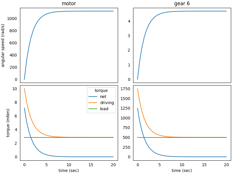
This plot is pretty crowded, and we are not interested in all time variables, so we can focus the plot only on interesting elements and variables. We can also specify a more convenient unit to use when plotting torques:
powertrain.plot(
    elements=['gear 6', motor],
    variables=['torque', 'driving torque', 'angular speed', 'load torque'],
    torque_unit='mNm',
    figsize=(8, 6)
)
See Powertrain.plot for
more details on method parameters.
Notice that we specified the elements either by the string name or by
instance name, both ways work. Also notice that the plot automatically
sorts:
the elements: the motor on the left and following elements proceeding to the right,
the time variables: kinematic variables at the top, then torques
grouped together in a single row and motor PWM in the last row.
We can see that at 10 seconds the angular speeds of motor and gear 6
are almost constant, confirming the insight previously mentioned by
analyzing the time snapshot: at 10 seconds the system is almost in a
stationary state.
We can see that, as the time passes, the driving torque on gear 6
equals the constant load torque and, as a result, the net torque on the
gear becomes close to zero.