5 - DC Motor PWM Control
System in Analysis
The complete example code is available
here.
The mechanical powertrain to be studied is the one described in the
4 - DC Motor Electric Analysis
example.
In that example, the motor absorbs its maximum electric current at the
start-up, 5 A, which may be too much for the system. Such a high current
may demagnetize the magnet inside the motor itself, so we want to keep
the absorbed current lower to prevent this issue. In order to do that,
we can control the motor supply voltage through the PWM.
This control can be also used to make the powertrain reach a specific
target position.
Model Set Up
We can start by limiting the start-up absorbed current through a rule that maintains the PWM proportional to the angular position of a gear, for example the gear 6, to which is attached an encoder that measure the gear angular position:
from gearpy.sensors import AbsoluteRotaryEncoder
from gearpy.motor_control.rules import StartProportionalToAngularPosition

encoder = AbsoluteRotaryEncoder(target=gear_6)

start_1 = StartProportionalToAngularPosition(
    encoder = encoder,
    powertrain=powertrain,
    target_angular_position=AngularPosition(10, 'rot'),
    pwm_min_multiplier=5
)
See
AbsoluteRotaryEncoder
and
StartProportionalToAngularPosition
for more details on instantiation parameters.
At the start-up the motor is supplied with a PWM that is 5 times its
minimum PWM, and it increases up to 1 when the gear 6 approaches 10
rotations from the reference position.
This rule has to be passed to the PWM control:
from gearpy.motor_control import PWMControl

motor_control_1 = PWMControl(powertrain=powertrain)
motor_control_1.add_rule(rule=start_1)
See PWMControl
for more details this class and its methods.
Simulation Set Up
The only modification to the simulation set up consist of passing the motor control object to the solver at simulation launch, the remaining set-ups stay the same:
solver = Solver(powertrain=powertrain)
solver.run(
    time_discretization=TimeInterval(0.5, 'sec'),
    simulation_time=TimeInterval(100, 'sec'),
    motor_control=motor_control_1
)
Results Analysis
We can get a general view of the system by plotting the time variables and focus the plot only on interesting elements and variables. We can also specify a more convenient unit to use when plotting torques:
powertrain.plot(
    figsize=(8, 10),
    elements=['motor', 'gear 6'],
    angular_position_unit='rot',
    torque_unit='mNm',
    variables=[
        'angular position',
        'angular speed',
        'angular acceleration',
        'driving torque',
        'load torque',
        'torque',
        'electric current',
        'pwm'
    ]
)
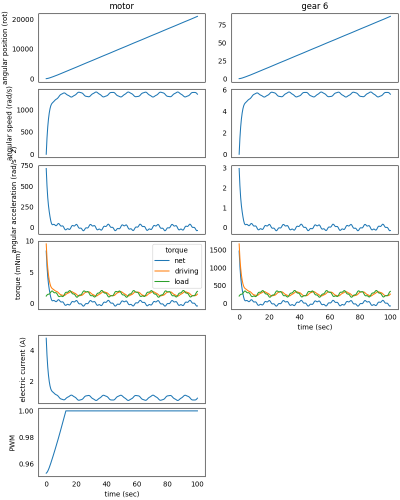
We can appreciate how the PWM starts from about 0.75 at the beginning of the simulation and increases up to 1 after about 15 seconds from the simulation start. At the same time, the electric current peak at the beginning of the simulation is decreased from 5 A to about 3.8 A, as desired.
Improved Model Set Up
However, this method is not so effective, since there still is an electric current peak and the electric current is not strictly controlled. If we can attach a tachometer to an element of the system, then we can replace the previous rule with another one, which lets us better control the electric current:
from gearpy.motor_control.rules import StartLimitCurrent
from gearpy.sensors import Tachometer

tachometer = Tachometer(target=motor)

start_2 = StartLimitCurrent(
    encoder=encoder,
    tachometer=tachometer,
    motor=motor,
    limit_electric_current=Current(2, 'A'),
    target_angular_position=AngularPosition(10, 'rot')
)
See Tachometer and
StartLimitCurrent
for more details on instantiation parameters.
This rule let us limit the maximum electric current absorbed by the
motor to 2 A up until the gear 6 (to which is attached the encoder)
reaches 10 rotations from the reference position.
Moreover, we want to add a second rule to make the gear 6 reach a
specific final position and stay there:
from gearpy.motor_control.rules import ReachAngularPosition

reach_position = ReachAngularPosition(
    encoder=encoder,
    powertrain=powertrain,
    target_angular_position=AngularPosition(40, 'rot'),
    braking_angle=Angle(10, 'rot')
)
See
ReachAngularPosition
for more details on instantiation parameters.
With this rule, the DC motor’s PWM is controlled in order to make the
gear 6 reach 40 rotations from the reference position and the whole
system will begin to brake 10 rotation before the target.
Finally, we have to add these two rules to a new motor control:
motor_control_2 = PWMControl(powertrain=powertrain)
motor_control_2.add_rule(rule=start_2)
motor_control_2.add_rule(rule=reach_position)
Simulation Set Up
We have to reset the previous simulation result and update the solver simulation parameters with the new motor control:
powertrain.reset()

solver.run(
    time_discretization=TimeInterval(0.5, 'sec'),
    simulation_time=TimeInterval(100, 'sec'),
    motor_control=motor_control_2
)
The remaining set-ups of the model stay the same.
Results Analysis
We can get the updated plot with the same code:
powertrain.plot(
    figsize=(8, 10),
    elements=['motor', 'gear 6'],
    angular_position_unit='rot',
    torque_unit='mNm',
    variables=[
        'angular position',
        'angular speed',
        'angular acceleration',
        'driving torque',
        'load torque',
        'torque',
        'electric current',
        'pwm'
    ]
)
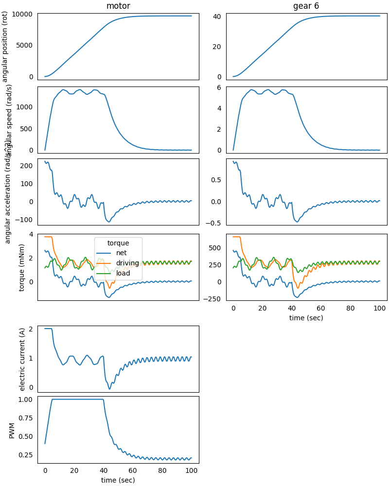
This time the PWM is controlled differently, and we can appreciate how
the electric current is always lower than 2 A at the beginning of the
simulation.
At 40 seconds from the simulation start, the system starts to brake in
order to reach the final position of the gear 6 at 40 rotations from
the reference position, as specified in the rule.