System in Analysis

The complete example code is available here.
The mechanical powertrain to be studied is reported in the image below:

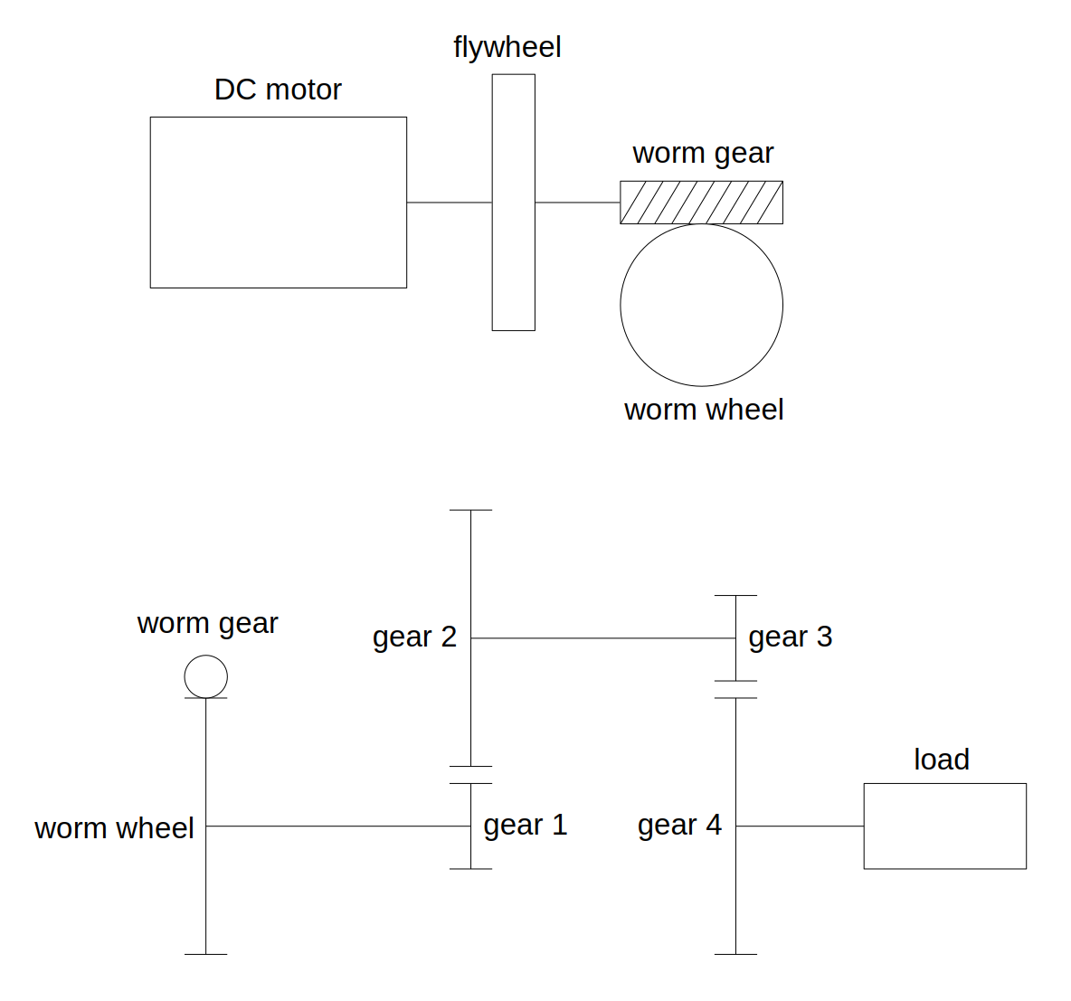
The flywheel and the worm gear are connected to the DC motor output shaft and rotate with it. The worm gear mates with the worm wheel, which is connected to gear 1 through a rigid shaft, so the worm wheel and the gear 1 rotate together. The gear 2 mates with gear 1 and is connected to gear 3 through a rigid shaft, so gear 2 and gear 3 rotate together. Finally, gear 3 mates with gear 4, which is connected to the external load.
gear 1, gear 2, gear 3 and gear 4 are helical gears.
The analysis is focused on powertrain elements kinematics, torques and stresses.

Model Set Up

As a first step, we instantiate the components of the mechanical powertrain:

from gearpy.mechanical_objects import (
    DCMotor,
    Flywheel,
    HelicalGear,
    WormGear,
    WormWheel)
from gearpy.units import (
    Angle,
    AngularSpeed,
    InertiaMoment,
    Length,
    Stress,
    Torque
)

motor = DCMotor(
    name = 'motor',
    no_load_speed=AngularSpeed(15000, 'rpm'),
    maximum_torque=Torque(10, 'mNm'),
    inertia_moment=InertiaMoment(3, 'gcm^2')
)
flywheel = Flywheel(
    name='flywheel',
    inertia_moment=InertiaMoment(20, 'kgcm^2')
)
worm_gear = WormGear(
    name='worm gear',
    n_starts=1,
    inertia_moment=InertiaMoment(3, 'gcm^2'),
    pressure_angle=Angle(20, 'deg'),
    helix_angle=Angle(10, 'deg'),
    reference_diameter=Length(10, 'mm')
)
worm_wheel = WormWheel(
    name='worm wheel',
    n_teeth=50,
    inertia_moment=InertiaMoment(500, 'gcm^2'),
    pressure_angle=Angle(20, 'deg'),
    helix_angle=Angle(10, 'deg'),
    module=Length(1, 'mm'),
    face_width=Length(10, 'mm')
)
gear_1 = HelicalGear(
    name='gear 1',
    n_teeth=10,
    inertia_moment= InertiaMoment(2, 'gcm^2'),
    helix_angle=Angle(20, 'deg'),
    module=Length(1, 'mm'),
    face_width=Length(15, 'mm'),
    elastic_modulus=Stress(200, 'GPa')
)
gear_2 = HelicalGear(
    name='gear 2',
    n_teeth=50,
    inertia_moment=InertiaMoment(750, 'gcm^2'),
    helix_angle=Angle(20, 'deg'),
    module=Length(1, 'mm'),
    face_width=Length(15, 'mm'),
    elastic_modulus=Stress(200, 'GPa')
)
gear_3 = HelicalGear(
    name='gear 3',
    n_teeth=10,
    inertia_moment=InertiaMoment(8, 'gcm^2'),
    helix_angle=Angle(20, 'deg'),
    module=Length(1.5, 'mm'),
    face_width=Length(20, 'mm'),
    elastic_modulus=Stress(200, 'GPa')
)
gear_4 = HelicalGear(
    name='gear 4',
    n_teeth=40,
    inertia_moment=InertiaMoment(2000, 'gcm^2'),
    helix_angle=Angle(20, 'deg'),
    module=Length(1.5, 'mm'),
    face_width=Length(20, 'mm'),
    elastic_modulus=Stress(200, 'GPa')
)

See WormGear, WormWheel and HelicalGear for more details on instantiation parameters.
Then it is necessary to specify the connection types between the components. We choose to study a non-ideal powertrain so, in order to take into account power loss in mating due to friction, we specify a gear mating efficiency below \(100\%\) and a friction coefficient in the worm gear mating:

from gearpy.utils import add_fixed_joint, add_gear_mating, add_worm_gear_mating

add_fixed_joint(master=motor, slave=flywheel)
add_fixed_joint(master=flywheel, slave=worm_gear)
add_worm_gear_mating(
    master=worm_gear,
    slave=worm_wheel,
    friction_coefficient=0.4
)
add_fixed_joint(master=worm_wheel, slave=gear_1)
add_gear_mating(master=gear_1, slave=gear_2, efficiency=0.9)
add_fixed_joint(master=gear_2, slave=gear_3)
add_gear_mating(master=gear_3, slave=gear_4, efficiency=0.9)

See add_fixed_joint, add_gear_mating and add_worm_gear_mating for more details.
We have to define the external load applied to gear 4. To keep the example simple, we can consider a constant load torque:

def ext_torque(time, angular_position, angular_speed):
    return Torque(500, 'mNm')

gear_4.external_torque = ext_torque

Finally, it is necessary to combine all components in a powertrain object:

from gearpy.powertrain import Powertrain

powertrain = Powertrain(motor=motor)

Simulation Set Up

Before performing the simulation, it is necessary to specify the initial condition of the system in terms of angular position and speed of the last gear in the mechanical powertrain. In this case we can consider the gear 4 still in the reference position:

from gearpy.units import AngularPosition

gear_4.angular_position = AngularPosition(0, 'rad')
gear_4.angular_speed = AngularSpeed(0, 'rad/s')

Finally, we have to set up the simulation parameters: the time discretization for the time integration and the simulation time. Now we are ready to run the simulation::

from gearpy.units import TimeInterval
from gearpy.solver import Solver

solver = Solver(powertrain=powertrain)
solver.run(
    time_discretization=TimeInterval(0.5, 'sec'), 
    simulation_time=TimeInterval(20, 'sec')
)

Results Analysis

We can get a snapshot of the system at a particular time of interest:

from gearpy.units import Time

powertrain.snapshot(
    target_time=Time(10, 'sec'),
    angular_position_unit='rot',
    torque_unit='mNm',
    driving_torque_unit='mNm',
    load_torque_unit='mNm'
)

Mechanical Powertrain Status at Time = 10 sec
            angular position (rot)  angular speed (rad/s)  angular acceleration (rad/s^2)  torque (mNm)  driving torque (mNm)  load torque (mNm) tangential force (N) bending stress (MPa) contact stress (MPa)  pwm
motor                  1750.283916            1212.664997                        0.158727      0.001448              2.279935           2.278487                                                                 1.0
flywheel               1750.283916            1212.664997                        0.158727      0.001448              2.279935           2.278487                                                                    
worm gear              1750.283916            1212.664997                        0.158727      0.001448              2.279935           2.278487             0.080352                                               
worm wheel               35.005678              24.253300                        0.003175      0.019617             30.883814          30.864198             1.235353            13.519356                          
gear 1                   35.005678              24.253300                        0.003175      0.019617             30.883814          30.864198              6.17284             1.697105            61.723522     
gear 2                    7.001136               4.850660                        0.000635      0.088274            138.977163         138.888889             5.559087             0.881963             58.57468     
gear 3                    7.001136               4.850660                        0.000635      0.088274            138.977163         138.888889            18.518519             2.545658            77.154403     
gear 4                    1.750284               1.212665                        0.000159      0.317788            500.317788         500.000000             16.67726             1.377898             73.21835                    

Notice that the load torque applied on the gear 4 is exactly the constant external torque we defined beforehand.
About 10 seconds after the simulation start, the driving torque applied on gear 4 is almost equal to the load torque on it, resulting in a very tiny angular acceleration. As a result, we can conclude that the system is almost in a stationary condition 10 seconds after the start.
We can get a more general view of the system by plotting the time variables of each element with respect to time:

powertrain.plot(
    figsize=(8, 8),
    elements=[motor, worm_gear, worm_wheel, gear_4],
    variables=[
        'angular position',
        'angular speed',
        'torque',
        'driving torque',
        'load torque',
        'bending stress',
        'contact stress'
    ],
    torque_unit='mNm'
)

We can see that at 10 seconds the angular speeds of motor and gear 4 are almost constant, confirming the insight previously mentioned by analyzing the time snapshot: at 10 seconds the system is almost in a stationary state.
As the time passes, the driving torque on gear 4 equals the constant load torque and, as a result, the net torque on the gear becomes close to zero.
Notice that the bending and contact stress are available for all gears and the bending stress has been computed for the worm wheel.