System in Analysis

The complete example code is available here.
The mechanical powertrain to be studied is the one described in the 5 - DC Motor PWM Control example.
In that example, the motor is controlled in order to keep the electric current absorption below a threshold and to make the gear 6 reach a specific final position and stay there.
After this simulation, we want to run a second simulation step, starting from the results of the first step. In this second step, the motor is still controlled in order to keep the current absorption below a threshold and to make the gear 6 reach another specific final position.
In order to analyze these steps, we need to concatenate two different simulation.

Second Step Model Set Up

After running the first step simulation, we can prepare the motor controls for the second step by setting up the electric current absorption limit to 2 A and the second target position for the gear 6 to 60 rotations from the reference position:

start_2 = StartLimitCurrent(
    encoder=encoder,
    tachometer=tachometer,
    motor=motor,
    limit_electric_current=Current(2, 'A'),
    target_angular_position=AngularPosition(50, 'rot')
)

reach_position_2 = ReachAngularPosition(
    encoder=encoder,
    powertrain=powertrain,
    target_angular_position=AngularPosition(60, 'rot'),
    braking_angle=Angle(10, 'rot')
)

motor_control_2 = PWMControl(powertrain=powertrain)
motor_control_2.add_rule(rule=start_2)
motor_control_2.add_rule(rule=reach_position_2)

Simulation Set Up

It is important to not reset the previous results, since we want to concatenate the new simulation results to these; so we only need to update the solver simulation parameters with the new motor control:

solver.run(
    time_discretization=TimeInterval(0.5, 'sec'),
    simulation_time=TimeInterval(100, 'sec'),
    motor_control=motor_control_2
)

The remaining set-ups of the model stay the same.

Results Analysis

We can get the updated plot with the same code:

powertrain.plot(
    figsize=(8, 10),
    elements=['motor', 'gear 6'],
    angular_position_unit='rot',
    torque_unit='mNm',
    variables=[
        'angular position',
        'angular speed',
        'angular acceleration',
        'driving torque',
        'load torque',
        'torque',
        'electric current',
        'pwm'
    ]
)

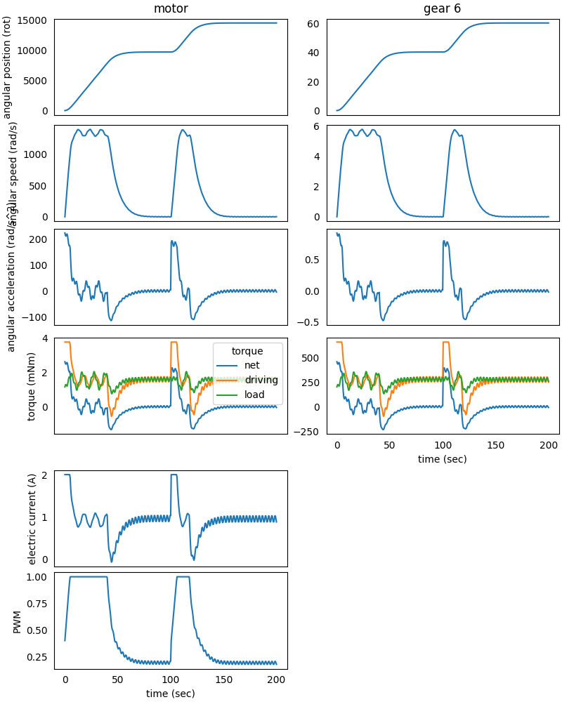
We can see the results of the first simulation up until 100 seconds from the start, where the powertrain starts up and make the gear 6 reach the destination at 40 rotations from the reference position, while keeping the motor electric current absorption below 2 A.
From 100 seconds up to the end, we can see the results from the second simulation, where the powertrain starts up again in order to make the gear 6 reach the second destination at 60 rotations from the reference position and still keeping the motor electric current absorption below 2 A.
The second step of the simulation depends on the first one only by the powertrain elements initial conditions (positions, speeds and accelerations); so the external load can be changed and also the solver parameters, like the simulation time and discretization.